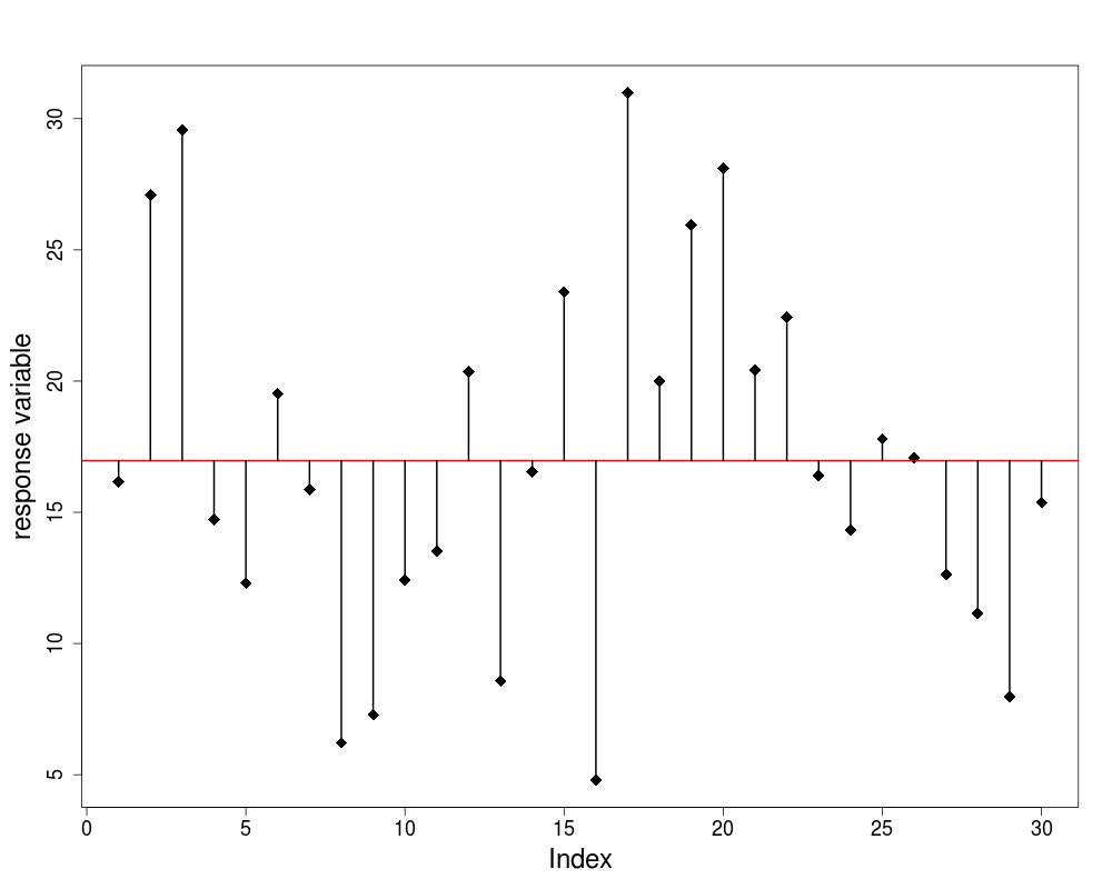
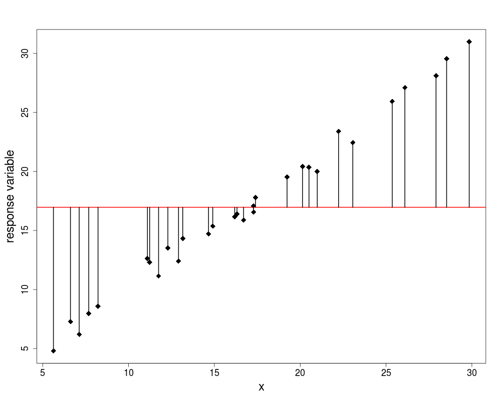
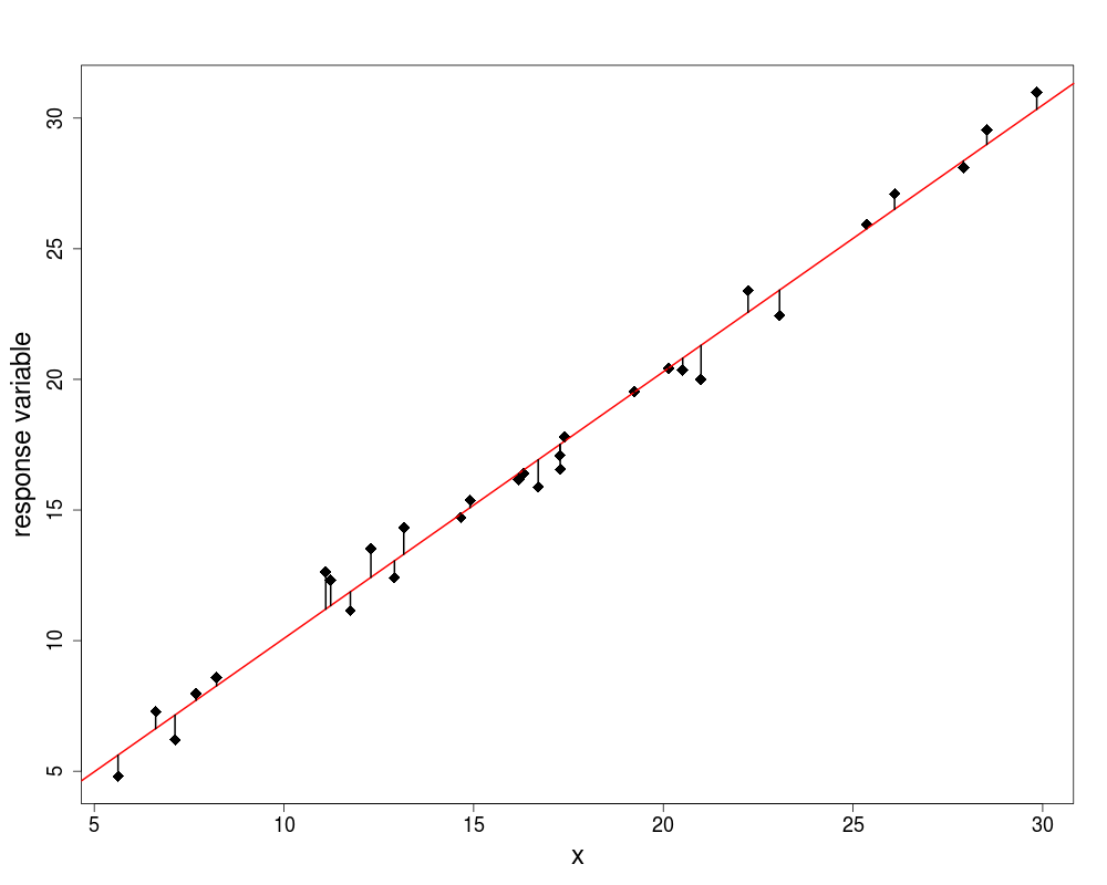
|
Größe: 12738
Kommentar:
|
Größe: 12470
Kommentar:
|
| Gelöschter Text ist auf diese Art markiert. | Hinzugefügter Text ist auf diese Art markiert. |
| Zeile 170: | Zeile 170: |
| Zeile 174: | Zeile 175: |
| == ANOVA == <img alt='sesssion2/img/fdens.png' src='-1' /> |
[[attachment:fdens.png|{{attachment:fdens.png||width=800,height=400}}]] |
| Zeile 180: | Zeile 183: |
| == ANOVA in R == | |
| Zeile 185: | Zeile 188: |
| == ANOVA in R == | |
| Zeile 194: | Zeile 197: |
| == ANOVA in R == | |
| Zeile 202: | Zeile 205: |
| == ANOVA in R == | |
| Zeile 225: | Zeile 228: |
| == ANOVA Assumptions == | === ANOVA Assumptions === |
| Zeile 228: | Zeile 231: |
| == Welch ANOVA == | === Welch ANOVA === |
| Zeile 239: | Zeile 242: |
| == Exercises - Solutions == | == Exercises and Solutions == |
| Zeile 242: | Zeile 245: |
| * install and load the granovaGG package (a package for visualization of ANOVAs), load the arousal data frame and use the stack() command to bring the data in the long form. Do a anova analysis. Is there a difference at least 2 of the groups? If indicated do a post-hoc test.\scriptsize | * install and load the granovaGG package (a package for visualization of ANOVAs), load the arousal data frame and use the stack() command to bring the data in the long form. Do a anova analysis. Is there a difference at least 2 of the groups? If indicated do a post-hoc test. |
| Zeile 261: | Zeile 264: |
| <img alt='sesssion2/img/aovgr1.png' src='-1' /> | [[attachment:aovgr1.png|{{attachment:aovgr1.png||width=800,height=400}}]] |
| Zeile 280: | Zeile 285: |
| <img alt='sesssion2/img/aovgr2.png' src='-1' /> \path[clip] (current page.north west) rectangle (current page.south east); * Coriolis acceleration \tikz[na] \node[coordinate] (n1) {}; * Transversal acceleration \tikz[na]\node [coordinate] (n2) {}; * Centripetal acceleration \tikz[na]\node [coordinate] (n3) {}; |
[[attachment:aovgr1.png|{{attachment:aovgr1.png||width=800,height=400}}]] |
Choosing the appropriate method
It is essential, therefore, that you can answer the following questions:
- Which of your variables is the response variable?
- Which are the explanatory variables?
- Are the explanatory variables continuous or categorical, or a mixture of both?
- What kind of response variable do you have: is it a continuous measurement, a count, a proportion, a time at death, or a category?
Choosing the appropriate method
Explanatory Variables are |
|
all continuous |
Regression |
all categorical |
Analysis of variance (ANOVA) |
both continuous and categorical |
Analysis of covariance (ANCOVA) |
Choosing the appropriate method
Response Variables |
|
(a) Continuous |
Normal regression, ANOVA or ANCOVA |
(b) Proportion |
Logistic regression |
(c) Count |
Log-linear models |
(d) Binary |
Binary logistic analysis |
(e) Time at death |
Survival analysis |
The best model is the model that produces the least unexplained variation (the minimal residual)
Choosing the appropriate method
- It is very important to understand that there is not one model;
- there will be a large number of different, more or less plausible models that might be fitted to any given set of data.
Maximum Likelihood
We define best in terms of maximum likelihood.
- given the data,
- and given our choice of model,
- what values of the parameters of that model make the observed data most likely?
We judge the model on the basis how likely the data would be if the model were correct.
Ockham's Razor
The principle is attributed to William of Ockham, who insisted that, given a set of equally good explanations for a given phenomenon, the correct explanation is the simplest explanation. The most useful statement of the principle for scientists is when you have two competing theories which make exactly the same predictions, the one that is simpler is the better.
Ockham's Razor
For statistical modelling, the principle of parsimony means that:
- models should have as few parameters as possible;
- linear models should be preferred to non-linear models;
- experiments relying on few assumptions should be preferred to those relying on many;
- models should be pared down until they are minimal adequate;
- simple explanations should be preferred to complex explanations.
Types of Models
Fitting models to data is the central function of R. There are no fixed rules and no absolutes. The object is to determine a minimal adequate model from a large set of potential models. For this reason we looking at the following types of models:
- the null model;
- the minimal adequate model;
- the maximal model; and
- the saturated model.
The Null model
- Just one parameter, the overall mean ybar
- Fit: none; SSE = SSY
- Degrees of freedom: n-1
- Explanatory power of the model: none
Adding Information
- model with

}}} parameters
- Fit: less than the maximal model, but not significantly so
- Degrees of freedom:

- Explanatory power of the model:

Adding Information
- model with

parameters
- Fit: less than the maximal model, but not significantly so
- Degrees of freedom:

- Explanatory power of the model:

Saturated/Maximal Model
saturated model
- One parameter for every data point
- Fit: perfect
- Degrees of freedom: none
- Explanatory power of the model: none
maximal model
- Contains all p factors, interactions and covariates that
- Degrees of freedom:

- Explanatory power of the model: it depends
How to choose...
- models are representations of reality that should be both accurate and convenient
- it is impossible to maximize a model’s realism, generality and holism simultaneously
- the principle of parsimony is a vital tool in helping to choose one model over another
- only include an explanatory variable in a model if it significantly improved the fit of the model (or if there other strong reasons)
- the fact that we went to the trouble of measuring something does not mean we have to have it in our model
ANOVA
- a technique we use when all explanatory variables are categorical (factor)
- if there is one factor with three or more levels we use one-way ANOVA (only two levels: t-test should be preferred, would give exactly the same answer since with 2 levels

- for more factors there there is two-way, three-way anova
- central idea is to compare two or more means by comparing variances
The Garden Data
A data frame with 14 observations on 2 variables.
- ozone: athmospheric ozone concentration
- garden: garden id
1 |
2 |
3 |
4 |
5 |
6 |
7 |
8 |
9 |
10 |
11 |
12 |
13 |
14 |
|
ozone |
9 |
7 |
6 |
8 |
5 |
11 |
9 |
11 |
9 |
6 |
10 |
8 |
8 |
12 |
garden |
a |
a |
a |
b |
a |
b |
b |
b |
b |
a |
b |
a |
a |
b |
Total Sum of Squares
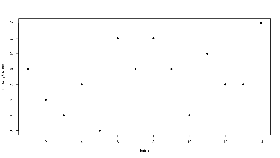
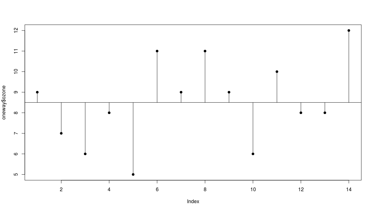
- we plot the values in order they are measured
Total Sum of Squares
- there is a lot of scatter, indicating that the variance in ozone is large
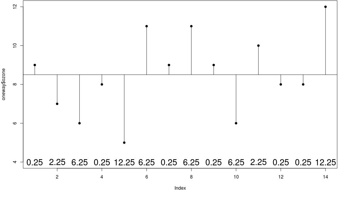
- to get a feel for the overall variance we plot the overall mean (8.5) and indicate each of the residuals by a vertical line
we refer to this overall variation as the total sum of squares, SSY or TSS
- in this case SSY = 55.5$
Group Means
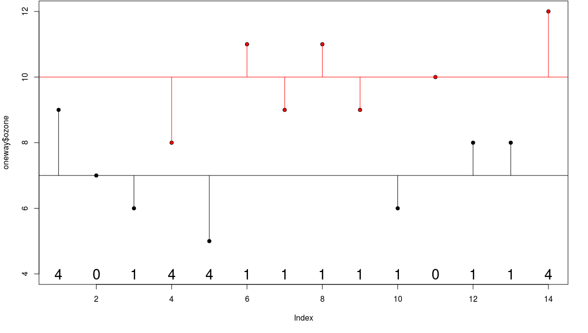
- now instead of fitting the overall mean, let us fit the individual garden means
garden |
a |
b |
mean |
7 |
10 |
Group Means
- now we see that the mean ozone concentration is substantially higher in garden B
- the aim of ANOVA is to determine
whether it is significantly higher or
- whether this kind of difference could come by chance alone
Error Sum of Squares
we define the new sum of squares as the error sum of squares (error in the sense of 'residual')
- in this case SSE = 24.0$
Treatment Sum of Squares
then the component of the variation that is explained by the difference of the means is called the treatment sum of squares SSA
- analysis of variance is based on the notion that we break down the total sum of squares into useful and informative components
- SSA = explained variation
- SSE = unexplained variation
ANOVA table
Source |
Sum of squares |
Degrees of freedom |
Mean square |
F ratio |
Garden |
31.5 |
1 |
31.5 |
15.75 |
Error |
24.0 |
12 |
s^2=2.0 |
|
Total |
55.5 |
13 |
|
ANOVA
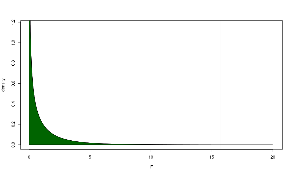
- now we need to test whether an F ratio of 15.75 is large or small
- we can use a table or software package
- I use here software to calculate the cumulative probability
ANOVA in R
- in R we use the lm() or the aov() command and
- the formula syntax a \sim b
- we assign this to an variable
   1 > m2 <- aov(ozone ~ garden, data=oneway)
   2 > m2
   3 garden Residuals
   4 Sum of Squares    31.5      24.0
   5 Residual standard error: 1.414214
   6 Estimated effects may be unbalanced
   7 > summary(m2)
   8 Df Sum Sq Mean Sq F value  Pr(>F)
   9 garden       1   31.5    31.5   15.75 0.00186 **
  10 Residuals   12   24.0     2.0
  11 > summary.lm(m2)
  12 Min     1Q Median     3Q    Max
  13 Estimate Std. Error t value Pr(>|t|)
  14 gardenb       3.0000     0.7559   3.969  0.00186 **
  15 Residual standard error: 1.414 on 12 degrees of freedom
  16 Multiple R-squared:  0.5676,    Adjusted R-squared:  0.5315
  17 > summary(m2)
  18 Df Sum Sq Mean Sq F value  Pr(>F)
  19 garden       1   31.5    31.5   15.75 0.00186 **
  20 Residuals   12   24.0     2.0
ANOVA Assumptions
- independed, normal distributed errors
- equality of variances (homogeneity)
Welch ANOVA
- generalization of the Welch t-test
- tests whether the means of the outcome variables are different across the factor levels
- assumes sufficiently large sample (greater than 10 times the number of groups in the calculation, groups of size one are to be excluded)
- sensitive to the existence of outliers (only few are allowed)
- the r command is oneway.test()
- non-parametric alternative kruskal.test()
* Look at the help of the TukeyHSD function. What is its purpose? * Execute the code of the example near the end of the help page, interpret the results! * install and load the granovaGG package (a package for visualization of ANOVAs), load the arousal data frame and use the stack() command to bring the data in the long form. Do a anova analysis. Is there a difference at least 2 of the groups? If indicated do a post-hoc test. * Visualize your results
Exercises and Solutions
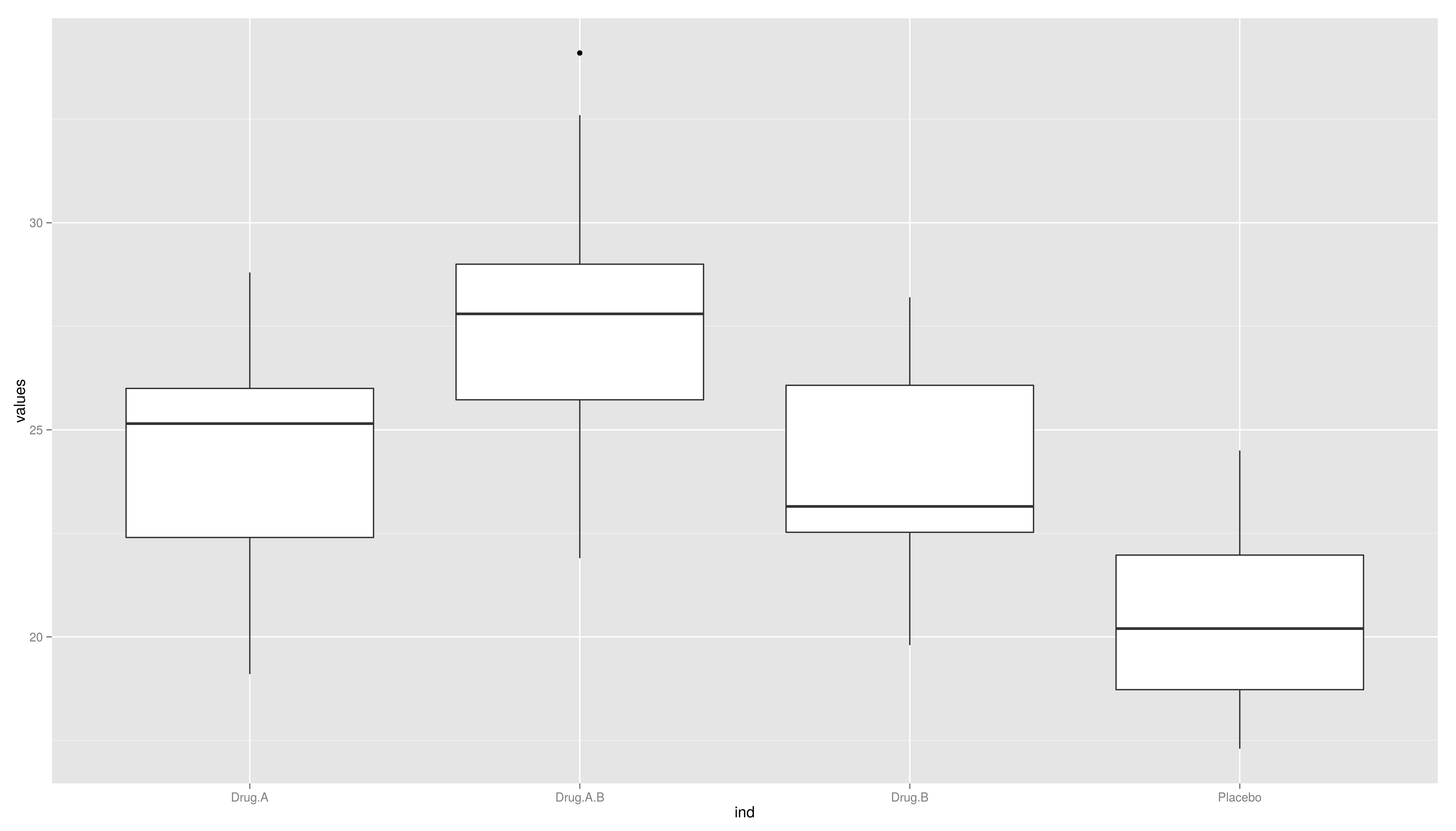
* Look at the help of the TukeyHSD function. What is its purpose? * Execute the code of the example near the end of the help page, interpret the results! * install and load the granovaGG package (a package for visualization of ANOVAs), load the arousal data frame and use the stack() command to bring the data in the long form. Do a anova analysis. Is there a difference at least 2 of the groups? If indicated do a post-hoc test.
   1 > require(granovaGG)
   2 > data(arousal)
   3 > datalong <- stack(arousal)
   4 > m1 <- aov(values ~ ind, data = datalong)
   5 > summary(m1)
   6 Df Sum Sq Mean Sq F value   Pr(>F)
   7 ind          3  273.4   91.13   10.51 4.17e-05 ***
   8 Residuals   36  312.3    8.68
   9 > TukeyHSD(m1)
  10 Tukey multiple comparisons of means
  11 diff           lwr        upr     p adj
* Visualize your results\scriptsize
   1 > granovagg.1w(datalong$values,group = datalong$ind)
   2 group group.mean trimmed.mean contrast variance standard.deviation
   3 4  Placebo      20.43        20.30    -3.65     5.83               2.41
   4 3   Drug.B      23.82        23.85    -0.26     7.50               2.74
   5 1   Drug.A      24.27        24.45     0.19     7.89               2.81
   6 2 Drug.A.B      27.81        27.52     3.73    13.49               3.67
   7 4         10
   8 3         10
   9 1         10
  10 2         10
  11 Below is a linear model summary of your input data
  12 Min     1Q Median     3Q    Max
  13 Estimate Std. Error t value Pr(>|t|)
  14 groupPlacebo   -3.8400     1.3172  -2.915  0.00608 **
  15 Residual standard error: 2.945 on 36 degrees of freedom
  16 Multiple R-squared:  0.4668,    Adjusted R-squared:  0.4223

