Unterschiede zwischen den Revisionen 9 und 11 (über 2 Versionen hinweg)

Classical Tests

Exercises

load the data (file: session4data.rdata)
make a new summary data frame (per subject and time) containing:
- the number of trials
- the number correct trials (absolute and relative)
- the mean TTime and the standard deviation of TTime
- the respective standard error of the mean
keep the information about Sex and Age_PRETEST
make a plot with time on the x-axis and TTime on the y-axis showing the means and the 95\% confidence intervals (geom_pointrange())
add the number of trials and the percentage of correct ones using geom_text()

Exercises - Solutions

load the data (file: session4data.rdata)
make a new summary data frame (per subject and time) containing:

   1 > sumdf <- data %>%
   2 +     group_by(Subject,Sex,Age_PRETEST,testid) %>%
   3 +     summarise(count=n(),
   4 +               n.corr = sum(Stim.Type=="hit"),
   5 +               perc.corr = n.corr/count,
   6 +               mean.ttime = mean(TTime),
   7 +               sd.ttime = sd(TTime),
   8 +               se.ttime = sd.ttime/sqrt(count))
   9 > head(sumdf)
  10 Subject Sex Age_PRETEST testid count n.corr perc.corr mean.ttime 
  11 1       1   f        3.11  test1    95     63 0.6631579   8621.674 
  12 2       1   f        3.11      1    60     32 0.5333333   9256.367 
  13 3       1   f        3.11      2    59     32 0.5423729   9704.712 
  14 4       1   f        3.11      3    60     38 0.6333333  14189.550 
  15 5       1   f        3.11      4    59     31 0.5254237  13049.831 
  16 6       1   f        3.11      5    59     33 0.5593220  14673.525 
  17 Variables not shown: sd.ttime se.ttime (dbl)

four possible situations

		Situation
		H_0 is true	H_0 is false
Conclusion	H_0 is not rejected	Correct decision	Type II error
Conclusion	H_0 is rejected	Type I error	Correct decision

Common symbols

n	number of observations (sample size)
K	number of samples (each having n elements)
alpha	level of significance
nu	degrees of freedom
mu	population mean
xbar	sample mean
sigma	standard deviation (population)
s	standard deviation (sample)
rho	population correlation coefficient
r	sample correlation coefficient
Z	standard normal deviate

Alternatives

The p-value is the probability of the sample estimate (of the respective estimator) under the null. The p-value is NOT the probability that the null is true.

Z-test for a population mean

The z-test is a something like a t-test (it is like you would know almost everything about the perfect conditions. It uses the normal distribution as distribution of the test statistic and is therefore a good example.

To investigate the significance of the difference between an assumed population mean

$\mu_0$

and a sample mean

$\bar{x}$

It is necessary that the population variance

$\sigma^2$

is known.

The test is accurate if the population values are normally distributed. If the population values are not normal, the test will still give an approximate guide.

Excercise

Write a function which takes a vector, the population standard deviation and the population mean as arguments and which gives the Z score as result.
- name the function ztest or my.z.test - not z.test because z.test is already used
- set a default value for the population mean
add a line to your function that allows you to process numeric vectors containing missing values!
the function pnorm(Z) gives the probability of

$x \leq Z$

Change your function so that it includes the p-value (for a two sided test) as result.

now let the result be a named vector containing the estimated difference, Z, p and the n.

You can always test your function using simulated values: rnorm(100,mean=0) gives you a vector containing 100 normal distributed values with mean 0.

Solutions

Write a function which takes a vector, the population standard deviation and the population mean as arguments and which gives the Z score as result.

   1 > ztest <- function(x,x.sd,mu=0){
   2 +     sqrt(length(x)) * (mean(x)-mu)/x.sd
   3 + }
   4 > set.seed(1)
   5 > ztest(rnorm(100),x.sd = 1)
   6 [1] 1.088874

Add a line to your function that allows you to also process numeric vectors containing missing values!

   1 > ztest <- function(x,x.sd,mu=0){
   2 +     x <- x[!is.na(x)]
   3 +     if(length(x) < 3) stop("too few values in x")
   4 +     sqrt(length(x)) * (mean(x)-mu)/x.sd
   5 + }

The function pnorm(Z) gives the probability of

$x \leq Z$

. Change your function so that it has the p-value (for a two sided test) as result.

   1 > ztest <- function(x,x.sd,mu=0){
   2 +     x <- x[!is.na(x)]
   3 +     if(length(x) < 3) stop("too few values in x")
   4 +     z <- sqrt(length(x)) * (mean(x)-mu)/x.sd
   5 +     2*pnorm(-abs(z))
   6 + }
   7 > set.seed(1)
   8 > ztest(rnorm(100),x.sd = 1)
   9 [1] 0.2762096

Now let the result be a named vector containing the estimated difference, Z, p and the n.

   1 > ztest <- function(x,x.sd,mu=0){
   2 +     x <- x[!is.na(x)]
   3 +     if(length(x) < 3) stop("too few values in x")
   4 +     est.diff <- mean(x)-mu
   5 +     z <- sqrt(length(x)) * (est.diff)/x.sd
   6 +     round(c(diff=est.diff,Z=z,pval=2*pnorm(-abs(z)),n=length(x)),4)
   7 + }
   8 > set.seed(1)
   9 > ztest(rnorm(100),x.sd = 1)
  10     diff        Z     pval        n 
  11   0.1089   1.0889   0.2762 100.0000

Requirements

Z-test for two population means (variances known and equal)
Z-test for two population means (variances known and unequal)

To investigate the statistical significance of the difference between an assumed population mean

$\mu_0$

and a sample mean

$\bar{x}$

. There is a function z.test() in the BSDA package

It is necessary that the population variance

$\sigma^2$

is known.

The test is accurate if the population is normally distributed. If the population is not normal, the test will still give an approximate guide.

Simulation Exercises

Now sample 100 values from a Normal distribution with mean 10 and standard deviation 2 and use a z-test to compare it against the population mean 10. What is the p-value?
Now do the sampling and the testing 1000 times, what would be the number of statistically significant results? Use replicate() (which is a wrapper of tapply()) or a for() loop! Record at least the p-values and the estimated differences! Use table() to count the p-vals below 0.05. What type of error do you associate with it? What is the smallest absolute difference with a p-value below 0.05?
Repeat the simulation above, change the sample size to 1000 in each of the 1000 samples! How many p-values below 0.05? What is now the smallest absolute difference with a p-value below 0.05?

Simulation Exercises -- Solutions

Now sample 100 values from a Normal distribution with mean 10 and standard deviation 2 and use a z-test to compare it against the population mean 10. What is the p-value? What the estimated difference?

   1 > ztest(rnorm(100,mean=10,sd=2),x.sd=2,mu=10)["pval"]
   2   pval
   3 0.0441    
   4 > ztest(rnorm(100,mean=10,sd=2),x.sd=2,mu=10)["diff"]
   5    diff 
   6 -0.0655 
   7 > ztest(rnorm(100,mean=10,sd=2),x.sd=2,mu=10)[c("pval","diff")]
   8   pval   diff 
   9 0.4515 0.1506

Now do the sampling and the testing 1000 times, what would be the number of statistically significant results? Use replicate() (which is a wrapper of tapply()) or a for() loop. Record at least the p-values and the estimated differences! Transform the result into a data frame.

Solution

using replicate()

   1 > res <- replicate(1000, ztest(rnorm(100,mean=10,sd=2),x.sd=2,mu=10))
   2 > res <- as.data.frame(t(res))
   3 > head(res)
   4 diff       Z   pval   n
   5 1 -0.2834 -1.4170 0.1565 100
   6 2  0.2540  1.2698 0.2042 100
   7 3 -0.1915 -0.9576 0.3383 100
   8 4  0.1462  0.7312 0.4646 100
   9 5  0.1122  0.5612 0.5747 100
  10 6 -0.0141 -0.0706 0.9437 100

using replicate() II

   1 > res <- replicate(1000, ztest(rnorm(100,mean=10,sd=2),x.sd=2,mu=10),
   2 +                        simplify = F)
   3 > res <- as.data.frame(Reduce(rbind,res))
   4 > head(res)
   5 diff       Z   pval   n
   6 init -0.0175 -0.0874 0.9304 100

using for()

   1 > res <- matrix(numeric(2000),ncol=2)
   2 > for(i in seq.int(1000)){
   3 +     res[i,] <- ztest(rnorm(100,mean=10,sd=2),x.sd=2,mu=10)[c("pval","diff")] }
   4 > res <- as.data.frame(res)
   5 > names(res) <- c("pval","diff")
   6 > head(res)
   7 pval    diff
   8 1 0.0591 -0.3775
   9 2 0.2466  0.2317
  10 3 0.6368  0.0944
  11 4 0.5538 -0.1184
  12 5 0.9897 -0.0026
  13 6 0.7748  0.0572

Use table() to count the p-vals below 0.05. What type of error do you associate with it? What is the smallest absolute difference with a p-value below 0.05?

   1 > table(res$pval < 0.05)
   2 FALSE  TRUE 
   3 960    40 
   4 > tapply(abs(res$diff),res$pval < 0.05,summary)
   5 $`FALSE`
   6    Min. 1st Qu.  Median    Mean 3rd Qu.    Max. 
   7  0.0002  0.0585  0.1280  0.1411  0.2068  0.3847 
   8 
   9 $`TRUE`
  10    Min. 1st Qu.  Median    Mean 3rd Qu.    Max. 
  11  0.3928  0.4247  0.4408  0.4694  0.5102  0.6859 
  12 
  13 > min(abs(res$diff[res$pval<0.05]))
  14 [1] 0.3928

Repeat the simulation above, change the sample size to 1000 in each of the 1000 samples! How many p-values below 0.05? What is now the smallest absolute difference with a p-value below 0.05?

   1 > res2 <- replicate(1000, ztest(rnorm(1000,mean=10,sd=2),
   2 +                              x.sd=2,mu=10))
   3 > res2 <- as.data.frame(t(res2))
   4 > head(res2)
   5      diff       Z   pval    n
   6 1 -0.0731 -1.1559 0.2477 1000
   7 2  0.0018  0.0292 0.9767 1000
   8 3  0.0072  0.1144 0.9089 1000
   9 4 -0.1145 -1.8100 0.0703 1000
  10 5 -0.1719 -2.7183 0.0066 1000
  11 6  0.0880  1.3916 0.1640 1000

Repeat the simulation above, change the sample size to 1000 in each of the 1000 samples! How many p-values below 0.05? What is now the smallest absolute difference with a p-value below 0.05?

   1 > table(res2$pval < 0.05)
   2 FALSE  TRUE 
   3 946    54 
   4 > tapply(abs(res2$diff),res$pval < 0.05,summary)
   5 $`FALSE`
   6    Min. 1st Qu.  Median    Mean 3rd Qu.    Max. 
   7 0.00010 0.02092 0.04285 0.05149 0.07400 0.22610 
   8 
   9 $`TRUE`
  10    Min. 1st Qu.  Median    Mean 3rd Qu.    Max. 
  11 0.00240 0.02115 0.04535 0.05435 0.08433 0.14760

Simulation Exercises Part II

Concatenate the both resulting data frames from above using rbind()
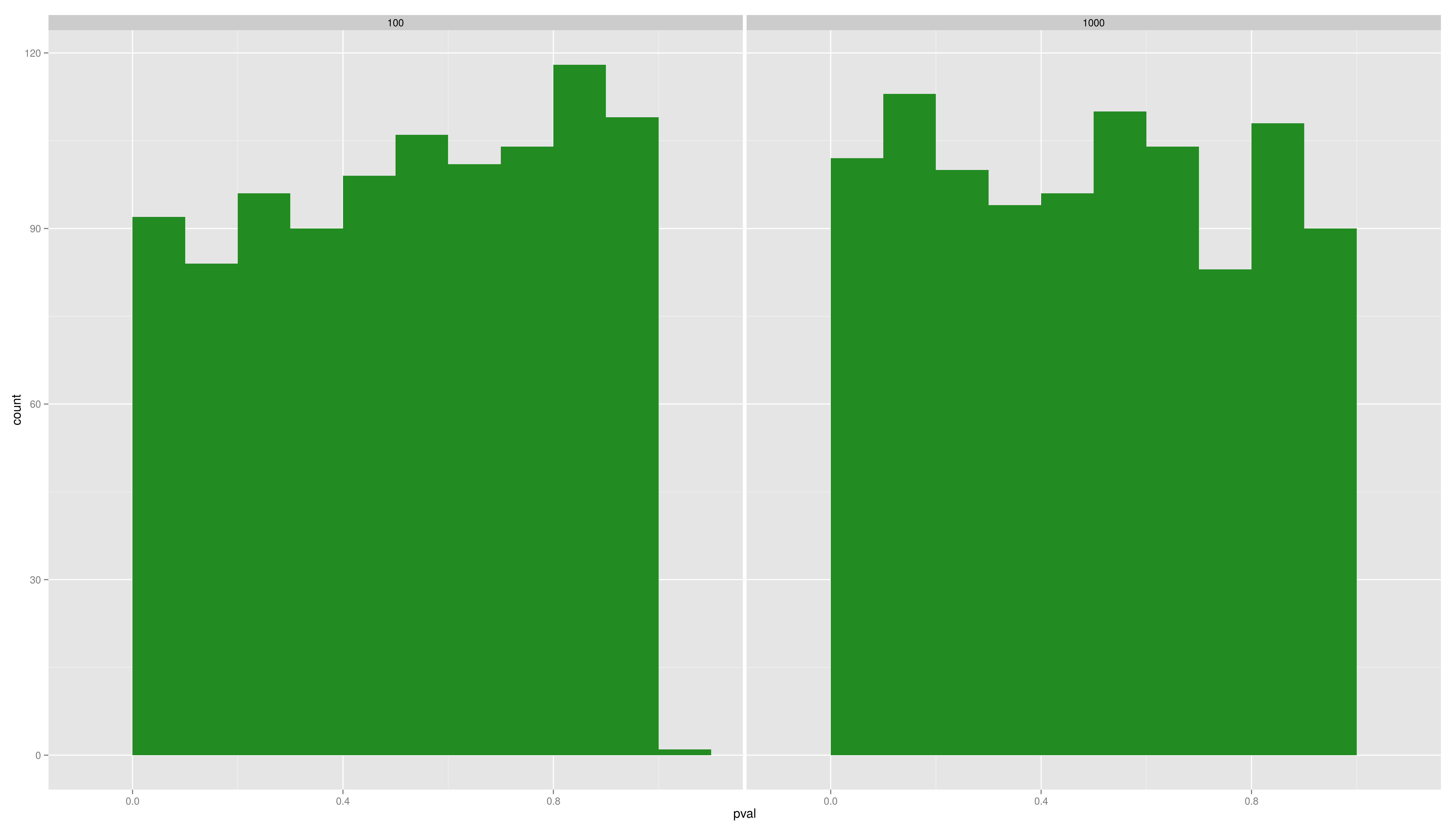
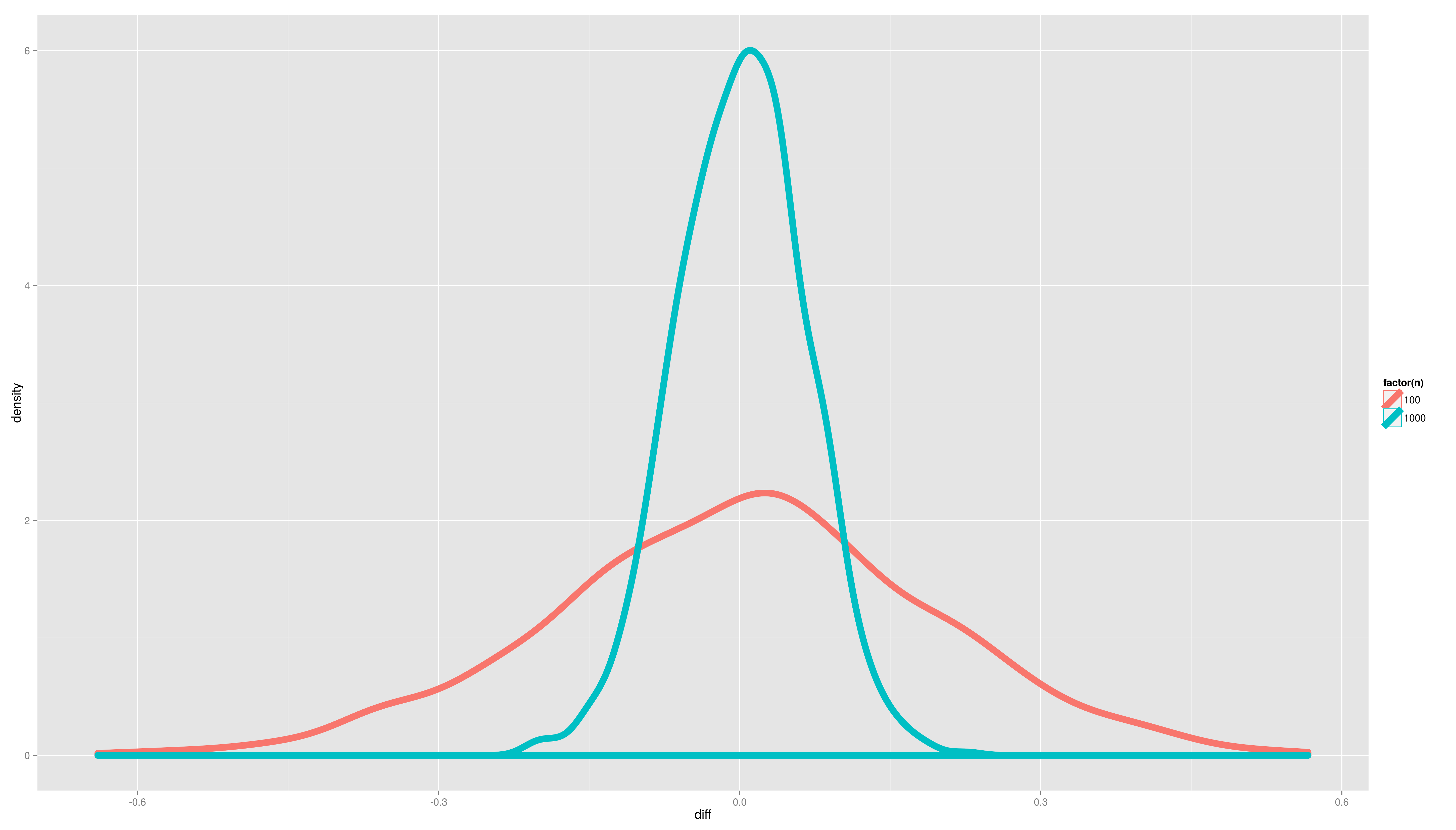
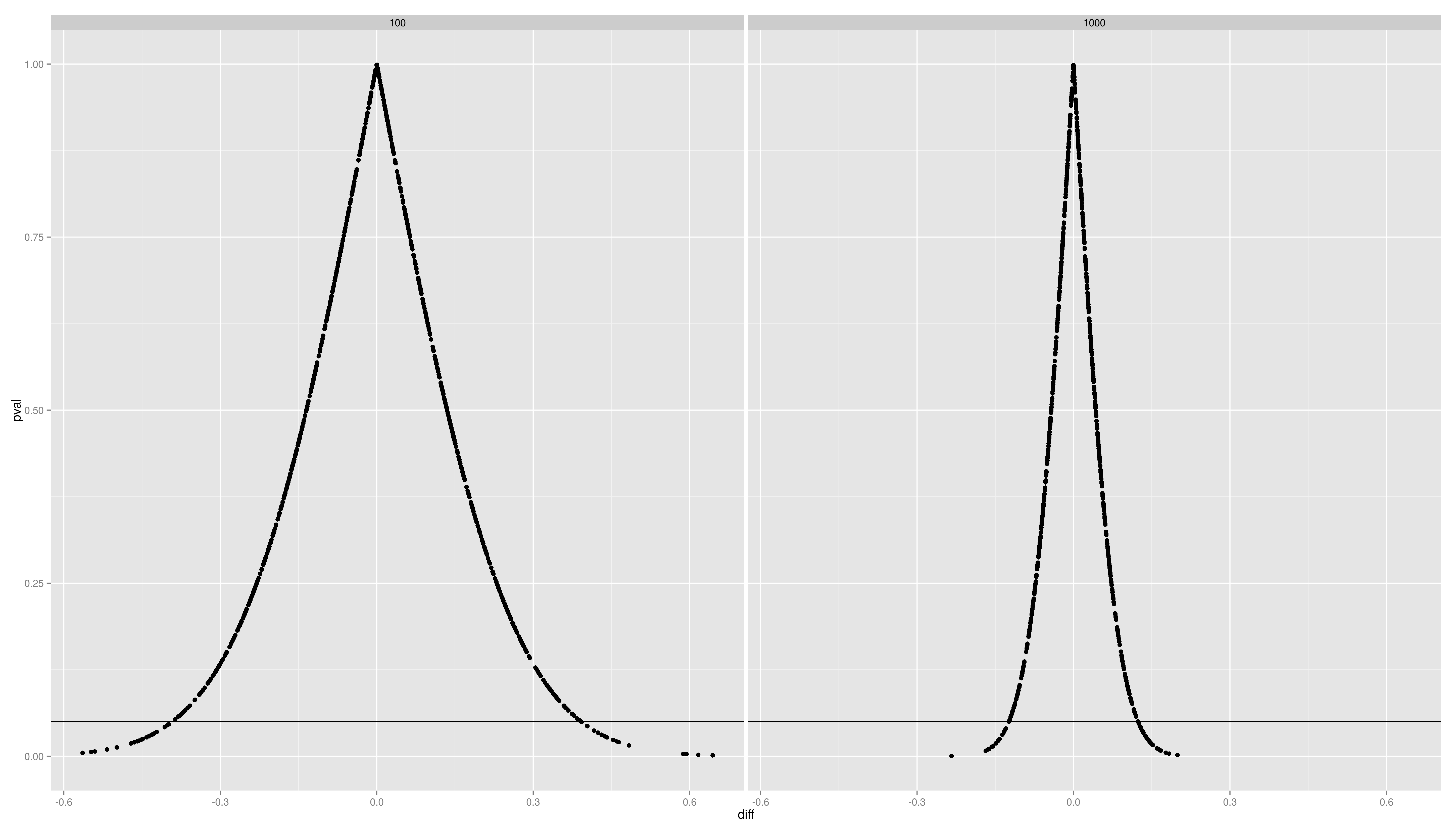
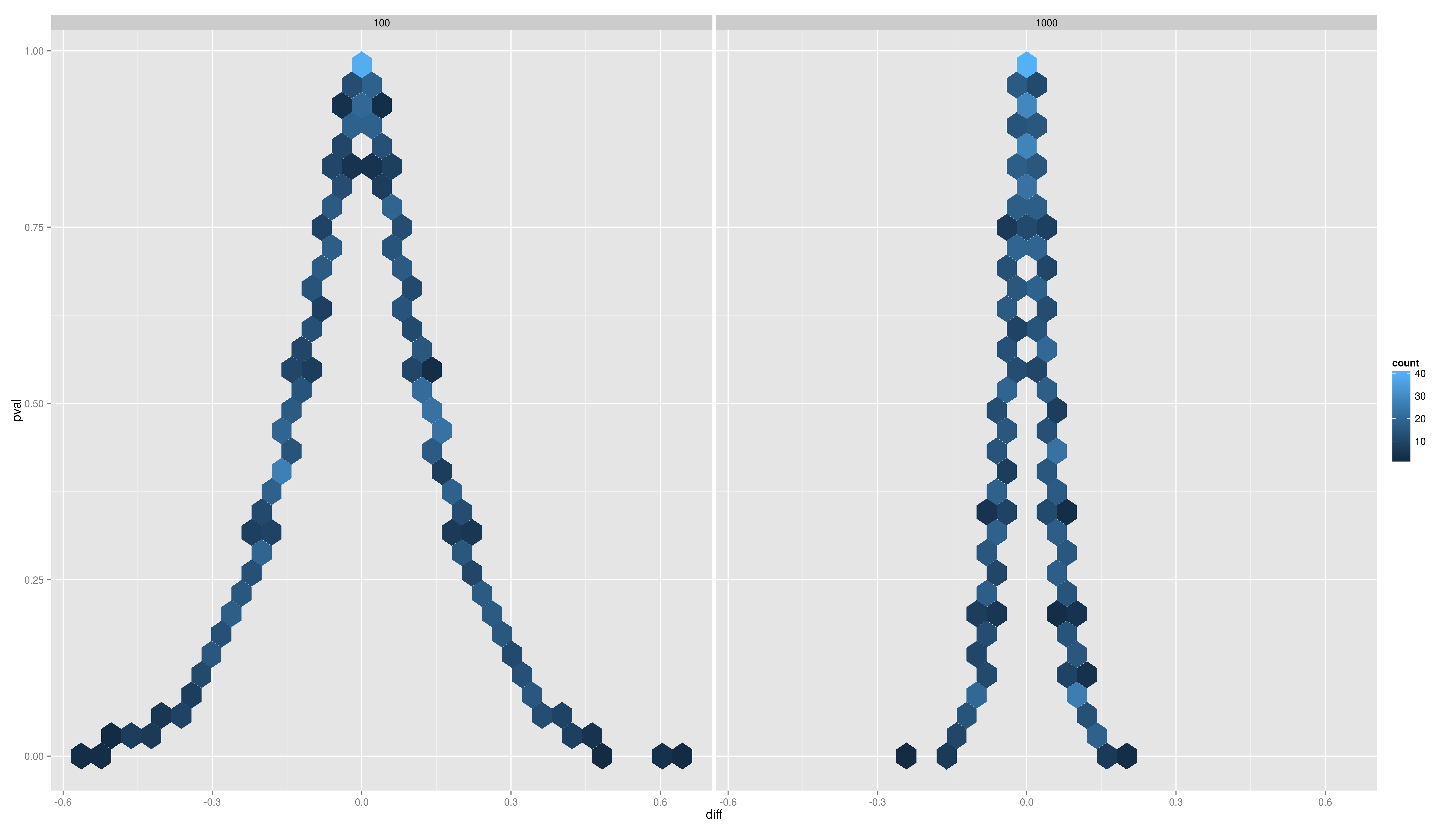
Plot the distributions of the pvals and the difference per sample size. Use ggplot2 with an appropriate geom (density/histogram)
What is the message?

Simulation Exercises -- Solutions

Concatenate the both resulting data frames from above using rbind()
Plot the distributions of the pvals and the difference per sample size. Use ggplot2 with an appropriate geom (density/histogram)

   1 > res <- rbind(res,res2)  
   2 > require(ggplot2)
   3 > ggplot(res,aes(x=pval)) +
   4 +     geom_histogram(bin=0.1,fill="forestgreen") +
   5 +     facet_grid(~ n)
   6 > ggsave("hist.png")

Plot the distributions of the pvals and the difference per sample size. Use ggplot2 with an appropriate geom (density/histogram)

   1 > ggplot(res,aes(x=diff,colour=factor(n))) +
   2 +     geom_density(size=3)
   3 > ggsave("dens.png")

Simulation Exercises -- Solutions

t-tests

A t-test is any statistical hypothesis test in which the test statistic follows a Student's t distribution if the null hypothesis is supported.

one sample t-test: test a sample mean against a population mean

$t = \frac{\bar{x}-\mu_0}{s/\sqrt{n}}$

where

$\bar{x}$

is the sample mean, s is the sample standard deviation and n is the sample size. The degrees of freedom used in this test is n-1

one sample t-test

   1 > set.seed(1)
   2 > x <- rnorm(12)
   3 > t.test(x,mu=0) ## population mean 0
   4 
   5         One Sample t-test
   6 
   7 data:  x
   8 t = 1.1478, df = 11, p-value = 0.2754
   9 alternative hypothesis: true mean is not equal to 0
  10 95 percent confidence interval:
  11  -0.2464740  0.7837494
  12 sample estimates:
  13 mean of x 
  14 0.2686377 
  15 
  16 > t.test(x,mu=1) ## population mean 1
  17 
  18         One Sample t-test
  19 
  20 data:  x
  21 t = -3.125, df = 11, p-value = 0.009664
  22 alternative hypothesis: true mean is not equal to 1
  23 95 percent confidence interval:
  24  -0.2464740  0.7837494
  25 sample estimates:
  26 mean of x 
  27 0.2686377

Two Sample t-tests

There are two ways to perform a two sample t-test in R:

given two vectors x and y containing the measurement values from the respective groups t.test(x,y)
given one vector x containing all the measurement values and one vector g containing the group membership

$t.test(x $\sim$ g)$

(read: x dependend on g)

Two Sample t-tests: two vector syntax

   1 > set.seed(1)
   2 > x <- rnorm(12)
   3 > y <- rnorm(12)
   4 > g <- sample(c("A","B"),12,replace = T)
   5 > t.test(x,y)
   6 > t.test(x,y)
   7 
   8         Welch Two Sample t-test
   9 
  10 data:  x and y
  11 t = 0.5939, df = 20.012, p-value = 0.5592
  12 alternative hypothesis: true difference in means is not equal to 0
  13 95 percent confidence interval:
  14  -0.5966988  1.0717822
  15 sample estimates:
  16  mean of x  mean of y 
  17 0.26863768 0.03109602

Two Sample t-tests: formula syntax

   1 > t.test(x ~ g)
   2 
   3         Welch Two Sample t-test
   4 
   5 data:  x by g
   6 t = -0.6644, df = 6.352, p-value = 0.5298
   7 alternative hypothesis: true difference in means is not equal to 0
   8 95 percent confidence interval:
   9  -1.6136329  0.9171702
  10 sample estimates:
  11 mean in group A mean in group B 
  12       0.1235413       0.4717726

Welch/Satterthwaite vs. Student

if not stated otherwise t.test() will not assume that the variances in the both groups are equal
if one knows that both populations have the same variance set the var.equal argument to TRUE to perform a student's t-test

Student's t-test

   1 > t.test(x, y, var.equal = T)
   2 
   3         Two Sample t-test
   4 
   5 data:  x and y
   6 t = 0.5939, df = 22, p-value = 0.5586
   7 alternative hypothesis: true difference in means is not equal to 0
   8 95 percent confidence interval:
   9  -0.5918964  1.0669797
  10 sample estimates:
  11  mean of x  mean of y 
  12 0.26863768 0.03109602

Requirements

the t-test, especially the Welch test is appropriate whenever the values are normally distributed
it is also recommended for group sizes > 30 (robust against deviation from normality)

Exercises

use a t-test to compare TTime according to Stim.Type, visualize it. What is the problem?
now do the same for Subject 1 on pre and post test (use filter() or indexing to get the resp. subsets)
use the following code to do the test on every subset Subject and testid, try to figure what is happening in each step:\tiny

   1 data.l <- split(data,list(data$Subject,data$testid),drop=T)
   2 tmp.l <- lapply(data.l,function(x) {
   3     if(min(table(x$Stim.Type)) < 5) return(NULL)
   4     tob <- t.test(x$TTime ~ x$Stim.Type)
   5     tmp <- data.frame(
   6         Subject = unique(x$Subject),
   7         testid = unique(x$testid),
   8         mean.group.1 = tob$estimate[1],
   9         mean.group.2 = tob$estimate[2],
  10         name.test.stat = tob$statistic,
  11         conf.lower = tob$conf.int[1],
  12         conf.upper = tob$conf.int[2],
  13         pval = tob$p.value,
  14         alternative = tob$alternative,
  15         tob$method)})
  16 res <- Reduce(rbind,tmp.l)

make plots to visualize the results.
how many tests have a statistically significant result? How many did you expect? Is there a tendency? What could be the next step?

Solutions

use a t-test to compare TTime according to Stim.Type, visualize it. What is the problem?

   1 > t.test(data$TTime ~ data$Stim.Type)
   2 
   3         Welch Two Sample t-test
   4 
   5 data:  data$TTime by data$Stim.Type
   6 t = -6.3567, df = 9541.891, p-value = 2.156e-10
   7 alternative hypothesis: true difference in means is not equal to 0
   8 95 percent confidence interval:
   9  -2773.574 -1466.161
  10 sample estimates:
  11       mean in group hit mean in group incorrect 
  12                17579.77                19699.64   
  13 
  14 > ggplot(data,aes(x=Stim.Type,y=TTime)) +
  15 +     geom_boxplot()

now do the same for Subject 1 on pre and post test (use filter() or indexing to get the resp. subsets)

   1 > t.test(data$TTime[data$Subject==1 & data$testid=="test1"] ~
   2 +        data$Stim.Type[data$Subject==1 & data$testid=="test1"])
   3 
   4         Welch Two Sample t-test
   5 
   6 data:  data$TTime[data$Subject == 1 & data$testid == "test1"] by data$Stim.Type[data$Subject == 1 & data$testid == "test1"]
   7 t = -0.5846, df = 44.183, p-value = 0.5618
   8 alternative hypothesis: true difference in means is not equal to 0
   9 95 percent confidence interval:
  10  -4930.842  2713.191
  11 
  12 sample estimates:
  13       mean in group hit mean in group incorrect 
  14                8248.175                9357.000 
  15 
  16 > t.test(data$TTime[data$Subject==1 & data$testid=="test2"] ~
  17 +        data$Stim.Type[data$Subject==1 & data$testid=="test2"])
  18         Welch Two Sample t-test
  19 
  20 data:  data$TTime[data$Subject == 1 & data$testid == "test2"] by data$Stim.Type[data$Subject == 1 & data$testid == "test2"]
  21 t = -1.7694, df = 47.022, p-value = 0.08332
  22 alternative hypothesis: true difference in means is not equal to 0
  23 95 percent confidence interval:
  24  -7004.4904   448.9388
  25 sample estimates:
  26       mean in group hit mean in group incorrect 
  27                4012.480                7290.256

make plots to visualize the results

   1 > ggplot(data,aes(x=testid,y=TTime)) +
   2 +    geom_boxplot(aes(fill=Stim.Type)) +
   3 +    facet_wrap(~Subject)
   4 > ggplot(data,aes(x=factor(Subject),y=TTime)) +
   5 +    geom_boxplot(aes(fill=Stim.Type)) +
   6 +    facet_wrap(~testid)

how many tests have an statistically significant result? How many did you expect?

   1 > table(res$pval < 0.05)
   2 FALSE  TRUE 
   3 165    22 
   4 > prop.table(table(res$pval < 0.05))
   5 
   6     FALSE      TRUE 
   7 0.8823529 0.1176471  
   8 >

Exercises - Solutions

What could be the next step?

   1 tmp.l <- lapply(data.l,function(x) {
   2     if(min(table(x$Stim.Type)) < 5) return(NULL)
   3     tob <- t.test(x$TTime ~ x$Stim.Type)
   4     tmp <- data.frame(
   5         Subject = unique(x$Subject),
   6         testid = unique(x$testid),
   7         perc.corr = sum(x$Stim.Type=="hit")/sum(!is.na(x$Stim.Type)),
   8         mean.group.1 = tob$estimate[1],
   9         mean.group.2 = tob$estimate[2],
  10         name.test.stat = tob$statistic,
  11         conf.lower = tob$conf.int[1],
  12         conf.upper = tob$conf.int[2],
  13         pval = tob$p.value,
  14         alternative = tob$alternative,
  15         tob$method)})
  16 
  17 res <- Reduce(rbind,tmp.l)
  18 
  19 ggplot(res,aes(x=perc.corr,y=mean.group.1 - mean.group.2)) +
  20     geom_point() +
  21     geom_smooth()

RstatisTik/RstatisTikPortal/RcourSe/CourseOutline/TestsInR (zuletzt geändert am 2015-05-03 06:24:36 durch mandy.vogel@googlemail.com)

-  ⇤ ← Revision 9 vom 2015-05-03 05:51:33 → 
  Größe: 18781
  Autor: mandy.vogel@googlemail.com
  Kommentar:
+   ← Revision 11 vom 2015-05-03 06:21:32 → ⇥
  Größe: 19597
  Autor: mandy.vogel@googlemail.com
  Kommentar:
-Gelöschter Text ist auf diese Art markiert.
+Hinzugefügter Text ist auf diese Art markiert.
 Zeile 64:
-The z-test is a something like a t-test (it is like you would know almost everything about the perfect conditions. It uses the normal distribution as test statistic and is therefore a good example.
To investigate the significance of the difference between an assumed population mean
+The z-test is a something like a t-test (it is like you would know almost everything about the perfect conditions. It uses the normal distribution as distribution of the test statistic and is therefore a good example.
 * To investigate the significance of the difference between an assumed population mean
 Zeile 72:
- * It is necessary that the population variance
+It is necessary that the population variance
 Zeile 75:
- * The test is accurate if the population is normally distributed. If the population is not normal, the test will still give an approximate guide.
+ * The test is accurate if the population values are normally distributed. If the population values are not normal, the test will still give an approximate guide.
 Zeile 83:
-$$x \leq Z$$ }}} . Change your function so that it has the p-value (for a two sided test) as result.
+$$x \leq Z$$ }}} Change your function so that it includes the p-value (for a two sided test) as result.
 Zeile 86:
-=== Z-test for a population mean - solution ===
+=== Solutions ===
 Zeile 132:
-diff        Z     pval        n
+    diff        Z     pval        n 
  0.1089   1.0889   0.2762 100.0000
-Zeile 156:
+Zeile 157:
-pval
+  pval
0.0441
-Zeile 158:
+Zeile 160:
-diff
+   diff 
-0.0655
-Zeile 160:
+Zeile 163:
-pval   diff
+  pval   diff 
0.4515 0.1506
-Zeile 164:
+Zeile 168:
-using replicate()
+=== Solution ===
 * using replicate()
-Zeile 178:
+Zeile 184:
-   * Now do the sampling and the testing 1000 times, what would be the number of statistically significant results? Use replicate() (which is a wrapper of tapply()) or a for() loop. Record at least the p-values and the estimated differences! Transform the result into a data frame.
using replicate() II
+ * using replicate() II
-Zeile 189:
+Zeile 195:
-   * Now do the sampling and the testing 1000 times, what would be the number of statistically significant results? Use replicate() (which is a wrapper of tapply()) or a for() loop. Record at least the p-values and the estimated differences! Transform the result into a data frame.
using for()
+ * using for()
-Zeile 213:
+Zeile 219:
+$`FALSE`
   Min. 1st Qu.  Median    Mean 3rd Qu.    Max. 
 0.0002  0.0585  0.1280  0.1411  0.2068  0.3847 

$`TRUE`
   Min. 1st Qu.  Median    Mean 3rd Qu.    Max. 
 0.3928  0.4247  0.4408  0.4694  0.5102  0.6859
-Zeile 223:
+Zeile 237:
-diff       Z   pval    n
+     diff       Z   pval    n
-Zeile 238:
+Zeile 252:
+$`FALSE`
   Min. 1st Qu.  Median    Mean 3rd Qu.    Max. 
0.00010 0.02092 0.04285 0.05149 0.07400 0.22610 

$`TRUE`
   Min. 1st Qu.  Median    Mean 3rd Qu.    Max. 
0.00240 0.02115 0.04535 0.05435 0.08433 0.14760
-Zeile 272:
+Zeile 293:
-{{{#!highlight r
> set.seed(1)
> x <- rnorm(12)
> t.test(x,mu=0) ## population mean 0
t = 1.1478, df = 11, p-value = 0.2754
alternative hypothesis: true mean is not equal to 0
95 percent confidence interval:
sample estimates:
mean of x 
}}}
{{{#!highlight r
> t.test(x,mu=1) ## population mean 1
t = -3.125, df = 11, p-value = 0.009664
alternative hypothesis: true mean is not equal to 1
95 percent confidence interval:
sample estimates:
mean of x 
}}}
-Zeile 301:
+Zeile 305:
+=== one sample t-test ===
-Zeile 347:
+Zeile 352:
+> t.test(x,y)

 Welch Two Sample t-test

data:  x and y
-Zeile 350:
+Zeile 360:
-sample estimates:
mean of x  mean of y
+ -0.5966988  1.0717822
sample estimates:
 mean of x  mean of y 
0.26863768 0.03109602
-Zeile 356:
+Zeile 368:
+ Welch Two Sample t-test

data:  x by g
-Zeile 359:
+Zeile 375:
+ -1.6136329  0.9171702
-Zeile 361:
+Zeile 378:
+.1235413       0.4717726
-Zeile 368:
+Zeile 386:
+ Two Sample t-test

data:  x and y
-Zeile 371:
+Zeile 393:
-sample estimates:
mean of x  mean of y
+ -0.5918964  1.0669797
sample estimates:
 mean of x  mean of y 
0.26863768 0.03109602
-Zeile 383:
+Zeile 407:
-tob <- t.test(x$TTime ~ x$Stim.Type)
tmp <- data.frame(
Subject = unique(x$Subject),
testid = unique(x$testid),
pval = tob$p.value,
alternative = tob$alternative,
+data.l <- split(data,list(data$Subject,data$testid),drop=T)
tmp.l <- lapply(data.l,function(x) {
    if(min(table(x$Stim.Type)) < 5) return(NULL)
    tob <- t.test(x$TTime ~ x$Stim.Type)
    tmp <- data.frame(
        Subject = unique(x$Subject),
        testid = unique(x$testid),
        mean.group.1 = tob$estimate[1],
        mean.group.2 = tob$estimate[2],
        name.test.stat = tob$statistic,
        conf.lower = tob$conf.int[1],
        conf.upper = tob$conf.int[2],
        pval = tob$p.value,
        alternative = tob$alternative,
        tob$method)})
-Zeile 465:
+Zeile 498:
-tob <- t.test(x$TTime ~ x$Stim.Type)
tmp <- data.frame(
Subject = unique(x$Subject),
testid = unique(x$testid),
pval = tob$p.value,
alternative = tob$alternative,
+tmp.l <- lapply(data.l,function(x) {
    if(min(table(x$Stim.Type)) < 5) return(NULL)
    tob <- t.test(x$TTime ~ x$Stim.Type)
    tmp <- data.frame(
        Subject = unique(x$Subject),
        testid = unique(x$testid),
        perc.corr = sum(x$Stim.Type=="hit")/sum(!is.na(x$Stim.Type)),
        mean.group.1 = tob$estimate[1],
        mean.group.2 = tob$estimate[2],
        name.test.stat = tob$statistic,
        conf.lower = tob$conf.int[1],
        conf.upper = tob$conf.int[2],
        pval = tob$p.value,
        alternative = tob$alternative,
        tob$method)})
-Zeile 472:
+Zeile 515:
-}}}
+ggplot(res,aes(x=perc.corr,y=mean.group.1 - mean.group.2)) +
    geom_point() +
    geom_smooth()
}}}

Quick Links

Search Wiki

Page Tools

Classical Tests

Exercises

Exercises - Solutions

four possible situations

Common symbols

Alternatives

Z-test for a population mean

Excercise

Solutions

Requirements

Simulation Exercises

Simulation Exercises -- Solutions

Solution

Simulation Exercises Part II

Simulation Exercises -- Solutions

Simulation Exercises -- Solutions

t-tests

one sample t-test

Two Sample t-tests

Two Sample t-tests: two vector syntax

Two Sample t-tests: formula syntax

Welch/Satterthwaite vs. Student

Student's t-test

Requirements

Exercises

Solutions

Exercises - Solutions