Unterschiede zwischen den Revisionen 1 und 3 (über 2 Versionen hinweg)

Introduction

Remember: Implicit Loops

A common application of loops is to apply a function to each element of a set of values and collect the results in a single structure. In R this is done by the functions:

lapply() - works on elements of a list
sapply() - same as lapply but simplify results
apply() - works on rows or colums of a matrix or a data frame (or more general on arrays)
tapply() - works on groups defined by an index

Exercises

Given the two R object m and l below use * use lapply() to get the class and the length of each element of l (two steps) * apply() to get the maximum of each column in m

   1 > m <- matrix(1:100, nrow=10)
   2 > l <- list(a=1:10,b=rep(c(T,F),2),c=letters)

read one file

   1 > file <- "../session1/session1data/pre001.txt"
   2 > pre1 <- read.file(file,skip=3)
   3 [1] "read ../session1/session1data/pre001.txt"
   4 > file <- "data/pretest/pre_001.txt"
   5 > pre1v2 <- read.file(file,skip=0)
   6 [1] "read ../session2/data/pretest/pre_001.txt"

read several files

we used dir() (with the arguments pattern, recursive, full.path) to get a list of file names we wanted to read in
we learned about lapply() which takes a list l and a function f to perform the function f on every element of the list l
so now we combine what we learned to read all files at once

get files names

   1 > files <- dir("../session2/data",full.names = T, 
   2 +                recursive = T,pattern = "[0-9]{3}\\.txt$")
   3 > files
   4 [1] "../session2/data/posttest/post_001.txt"   
   5 [2] "../session2/data/posttest/post_002.txt"   
   6 [3] "../session2/data/posttest/post_003.txt"   
   7 [4] "../session2/data/posttest/post_004.txt"   
   8 [5] "../session2/data/posttest/post_005.txt"   
   9 [6] "../session2/data/posttest/post_006.txt"   
  10 [7] "../session2/data/posttest/post_007.txt"

read in files

source the file containing our function read.file()
use lapply() to use read.file() on every entry of the list of file names

   1 > source("function.r")
   2 > df.list <- lapply(files,read.file,skip=0)
   3 [1] "read ../session2/data/posttest/post_001.txt"
   4 [1] "read ../session2/data/posttest/post_002.txt"
   5 [1] "read ../session2/data/posttest/post_003.txt"
   6 [1] "read ../session2/data/posttest/post_004.txt"
   7 [1] "read ../session2/data/posttest/post_005.txt"
   8 [1] "read ../session2/data/posttest/post_006.txt"
   9 [1] "read ../session2/data/posttest/post_007.txt"
  10 [1] "read ../session2/data/posttest/post_008.txt"

Result

what we get is a list df.list containing the results: every element of the list is a data frame if read.file() read in successfully the respective file
so our variable files contains 195 file names

   1 > length(files)
   2 [1] 195

so df.list contains 195 elements

   1 > length(df.list)
   2 [1] 195

we can check the class of each of these results again with sapply()

   1 > table(sapply(df.list,class))
   2 192          2

Remember: Combining Data Frames

We learned about three basis functions to combine data frame

rbind() - combine two data frames row wise
cbind() - combine two data frames column wise
merge() - combine two data with respect two one or more identifying columns
all of them are binary function
so you can not put more than two data frame into it
using only these function it would be a tedious and boring work to combine 192 data frames

Reduce()

is also a higher order function (functional)
Reduce() uses a binary function (like rbind() or merge()) to combine successively the elements of a given list
it can be used if you have not only two but many data frames

Example

first we make up 4 artifical data frames

   1 > (d1 <- data.frame(id=LETTERS[c(1,2,3)],day1=sample(10,3)))
   2 id day1
   3 1  A    3
   4 2  B    1
   5 3  C    7
   6 > (d2 <- data.frame(id=LETTERS[c(1,3,5,6)],day2=sample(10,4)))
   7 id day2
   8 1  A    8
   9 2  C    2
  10 3  E    5
  11 4  F    3
  12 > (d3 <- data.frame(id=LETTERS[c(2,4:6)],day3=sample(10,4)))
  13 id day3
  14 1  B    8
  15 2  D    3
  16 3  E    4
  17 4  F   10
  18 > (d4 <- data.frame(id=LETTERS[c(1:5)],day4=sample(10,5)))
  19 id day4
  20 1  A    2
  21 2  B    7
  22 3  C    8
  23 4  D    9
  24 5  E    1

now we use Reduce() in combination with merge()

   1 > Reduce(merge,list(d1,d2,d3,d4))
   2 [1] id   day1 day2 day3 day4

and what we get is an empty data frame
well this isn't exactly what we wanted, so why?
it is because the default behavior of merge() is set all=F, so we get only complete lines which is in this case - none
so we have to define a wrapper function which only change this argument to all=T
set all to TRUE

   1 > Reduce(function(x,y) { merge(x,y, all=T) },
   2 +        list(d1,d2,d3,d4))
   3 id day1 day2 day3 day4
   4 1  A    3    8   NA    2
   5 2  B    1   NA    8    7
   6 3  C    7    2   NA    8
   7 4  E   NA    5    4    1
   8 5  F   NA    3   10   NA
   9 6  D   NA   NA    3    9

which is exactly what we want
a second example in combination with rbind()

   1 > d4$day <- names(d4)[2]
   2 > names(d4)[2] <- "score"
   3 > Reduce(function(x,y) { y$day <- names(y)[2]
   4 +                        names(y)[2] <- "score"
   5 +                        rbind(x,y) } ,
   6 +        list(d1,d2,d3), init = d4)
   7 id score  day
   8 1   A     2 day4
   9 2   B     7 day4
  10 3   C     8 day4
  11 4   D     9 day4

which is exactly what we want

Reduce() Exercise

the list ml contains three vectors
use lapply() to get the class of each of them
then use Reduce() and combination with c() to coerce them into one vector. Of which class is the resulting vector?

   1 > ml <- list(vl <- c(TRUE,FALSE),
   2 +            vn <- 1:10,
   3 +            vc <- letters)

solution

use lapply() to get the class of each of them

   1 > lapply(ml,class)
   2 [1] "logical"
   3 [1] "integer"
   4 [1] "character"

then use Reduce() and combination with c() to coerce them into one vector. Of which class is the resulting vector?

   1 > rv <- Reduce(c,ml)
   2 > rv
   3 [1] "1"  "0"  "1"  "2"  "3"  "4"  "5"  "6"  "7"  "8"  "9"  "10" "a"  "b"  "c" 
   4 [16] "d"  "e"  "f"  "g"  "h"  "i"  "j"  "k"  "l"  "m"  "n"  "o"  "p"  "q"  "r" 
   5 [31] "s"  "t"  "u"  "v"  "w"  "x"  "y"  "z" 
   6 > class(rv)
   7 [1] "character"

Combine all data frames

We used lapply() and our function read.file() to read all files in files
and we got back a list df.list containing 192 data frames

   1 > df.list <- lapply(files,read.file,skip=0)
   2 [1] "read data/posttest/post_001.txt"
   3 [1] "read data/posttest/post_002.txt"
   4 [1] "read data/posttest/post_003.txt"
   5 [1] "read data/posttest/post_004.txt"
   6 [1] "read data/posttest/post_005.txt"
   7 > table(sapply(df.list,class))
   8 192          3

Combine all data frames - exercise

now use what we learned about Reduce{} and combining data frames using rbind() to combine these 192 data frames.

solution

   1 > data <- Reduce(rbind,df.list)
   2 > nrow(data)
   3 [1] 12704
   4 > table(data$Subject)
   5 001_test2 002_test2 003_test2 004_test2 005_test2 006_test2 007_test2 008_test2 
   6 93        91        96        93        95        95        93        96 
   7 009_test2 010_test2 011_test2 012_test2 013_test2 014_test2 015_test2 016_test2 
   8 92        94        95        96        96        95        96        94 
   9 017_test2 018_test2 019_test2 020_test2 001_test1 002_test1 003_test1 004_test1 
  10 95        94        96        95        95        95        96        94 
  11 005_test1 006_test1 007_test1 008_test1 009_test1 010_test1 011_test1 012_test1 
  12 96        95        94        90        96        95        91        96 
  13 013_test1 014_test1 015_test1 016_test1 017_test1 018_test1 019_test1 020_test1 
  14 95        96        95        91        96        96        96        96 
  15 001_1     002_1     003_1     004_1     005_1     006_1    CHGU_1    008_1a 
  16 60        59        60        54        60        59        60        60 
  17 009_1     010_1     RMK_1     013_1     014_1     015_1     016_1    IJ2K_1 
  18 60        60        59        59        60        58        59        58 
  19 018_1     019_1     020_1     001_2     002_2     003_2     004_2     005_2 
  20 60        59        60        59        59        57        58        57 
  21 006_2     007_2     008_2     009_2     010_2     011_2     012_2     013_2 
  22 58        58        54        58        58        59        59        56 
  23 014_2     015_2     016_2     017_2     018_2     019_2     020_2     001_3

The Function no 2

so it is recommended to build again a function out of this

   1 > read.files <- function(filesdir,skip=3,recursive=F,pattern="."){
   2 +     files <- dir(filesdir,
   3 +                  full.names = T,
   4 +                  recursive = recursive,
   5 +                  pattern = pattern)
   6 +     Reduce(rbind,lapply(files,read.file,skip=skip))}
   7 > data <- read.files("data",recursive = T,skip=0,pattern = "\\.txt$")
   8 [1] "read data/posttest/post_001.txt"
   9 [1] "read data/posttest/post_002.txt"
  10 [1] "read data/posttest/post_003.txt"
  11 [1] "read data/posttest/post_004.txt"
  12 [1] "read data/posttest/post_005.txt"

by changing the pattern (passed through to dir() we can limit the read in files to specific time or person\tiny

   1 > sub1 <- read.files("../session2/data",
   2 +                    skip = 0, recursive = T,pattern="\\002\\.txt$")
   3 [1] "read ../session2/data/posttest/post_002.txt"
   4 [1] "read ../session2/data/pretest/pre_002.txt"
   5 [1] "read ../session2/data/training_1/train_002.txt"
   6 [1] "read ../session2/data/training_2/train_002.txt"
   7 [1] "read ../session2/data/training_3/train_002.txt"
   8 > test <- read.files("../session2/data",
   9 +                    skip = 0, recursive = T,pattern="p[ro].+\\.txt$")
  10 [1] "read ../session2/data/posttest/post_001.txt"
  11 [1] "read ../session2/data/posttest/post_002.txt"
  12 [1] "read ../session2/data/pretest/pre_001.txt"
  13 [1] "read ../session2/data/pretest/pre_002.txt"

The Subject column

table the Subject column again. What is the problem?

   1 > table(data$Subject)
   2 001_test2 002_test2 003_test2 004_test2 005_test2 006_test2 007_test2 008_test2 
   3 93        91        96        93        95        95        93        96 
   4 009_test2 010_test2 011_test2 012_test2 013_test2 014_test2 015_test2 016_test2 
   5 92        94        95        96        96        95        96        94 
   6 017_test2 018_test2 019_test2 020_test2 001_test1 002_test1 003_test1 004_test1 
   7 95        94        96        95        95        95        96        94

subject and time coded in one variable
we create two new variables using the str_split() function (stringr package)
because str_split() has a list containing a vector as result we have to use it in combination with sapply()
then correct some of the person ids

   1 > data$persid <- sapply(data$Subject,function(x)
   2 +     str_split(x,pattern = "_")[[1]][1])
   3 > data$testid <- sapply(data$Subject,function(x)
   4 +     str_split(x,pattern = "_")[[1]][2])

a alternative is using again regular expressions using the str_replace() function (again stringr package)
str_replace() takes three arguments: the string, the pattern to be replaced and the replacement

   1 > data$testid <- str_replace(data$Subject,"^.+_","")
   2 > data$persid <- str_replace(data$Subject,"_.+$","")
   3 > data$Subject <- NULL

now table the personid column
what is left to do?

   1 > table(data$persid)
   2 001  002  003  004  005  006  007  008  009  010  011  012  013  014  015  016 
   3 665  662  666  587  608  588  600  654  536  543  600  523  589  669  662  663 
   4 017  018  019  020 CHGU GA3K IJ2K Kj6K  RMK 
   5 604  668  667  656   60   58   58   59   59 
   6 > data$persid[data$persid=="CHGU"] <- "007"

The Subject column Exercises

there are some more wrong person ids: RMK - 011, IJ2K - 017, GA3K - 004, Kj6K - 006. Correct them!

solution

   1 > data$persid[data$persid=="RMK"] <- "011"
   2 > data$persid[data$persid=="IJ2K"] <- "017"
   3 > data$persid[data$persid=="GA3K"] <- "004"
   4 > data$persid[data$persid=="Kj6K"] <- "006"

Merging

* now read in the file subjectsdemographics.txt using the appropriate command * join the demographics with our data data frame (there is a little problem left - compare the persid and Subject columns)

   1 > persdat <- read.table("data/subjectdemographics.txt",
   2 +                       sep="\t",
   3 +                       header=T)
   4 > persdat$Subject
   5 [1]  1  2  3  4  5  6  7  8  9 10 11 12 13 14 15 16 17 18 19 20
   6 > unique(data$persid)
   7 [1] "001" "002" "003" "004" "005" "006" "007" "008" "009" "010" "011" "012"
   8 [13] "013" "014" "015" "016" "017" "018" "019" "020"
   9 > data$persid <- as.numeric(data$persid)
  10 > unique(data$persid)
  11 [1]  1  2  3  4  5  6  7  8  9 10 11 12 13 14 15 16 17 18 19 20
  12 > data <- merge(persdat,data,by.x = "Subject",by.y = "persid",all=T)
  13 > head(data)
  14 > summary(data)
  15 Subject      Sex       Age_PRETEST        Trial          Event.Type   
  16 1st Qu.: 5.00   m:5046   1st Qu.:3.110   1st Qu.:112.0   Response:12704  
  17 Median :11.00            Median :4.400   Median :222.0   Sound   :    0  
  18 Mean   :10.53            Mean   :4.154   Mean   :223.1   Pause   :    0  
  19 3rd Qu.:16.00            3rd Qu.:4.600   3rd Qu.:332.0   Resume  :    0

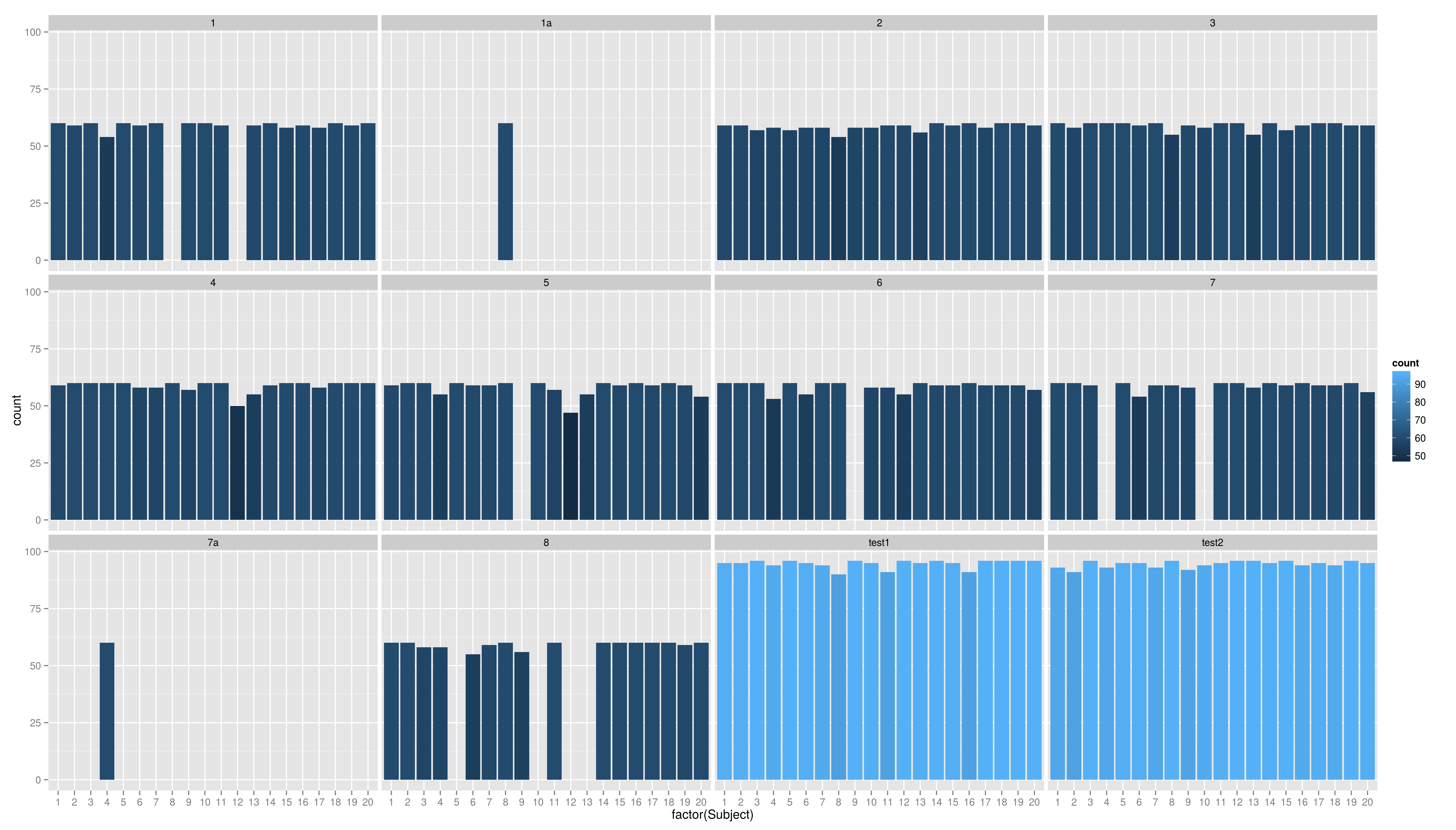
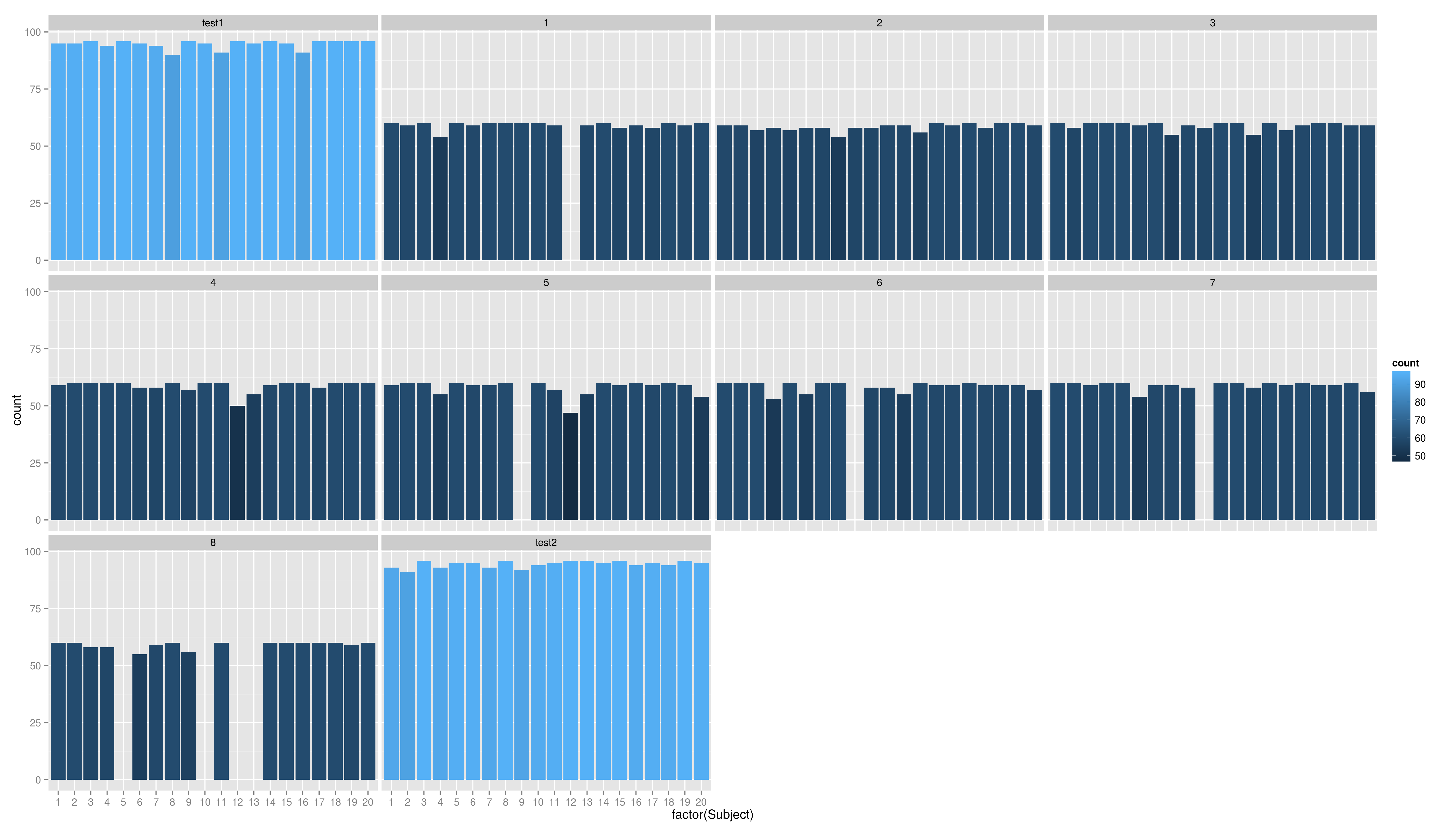
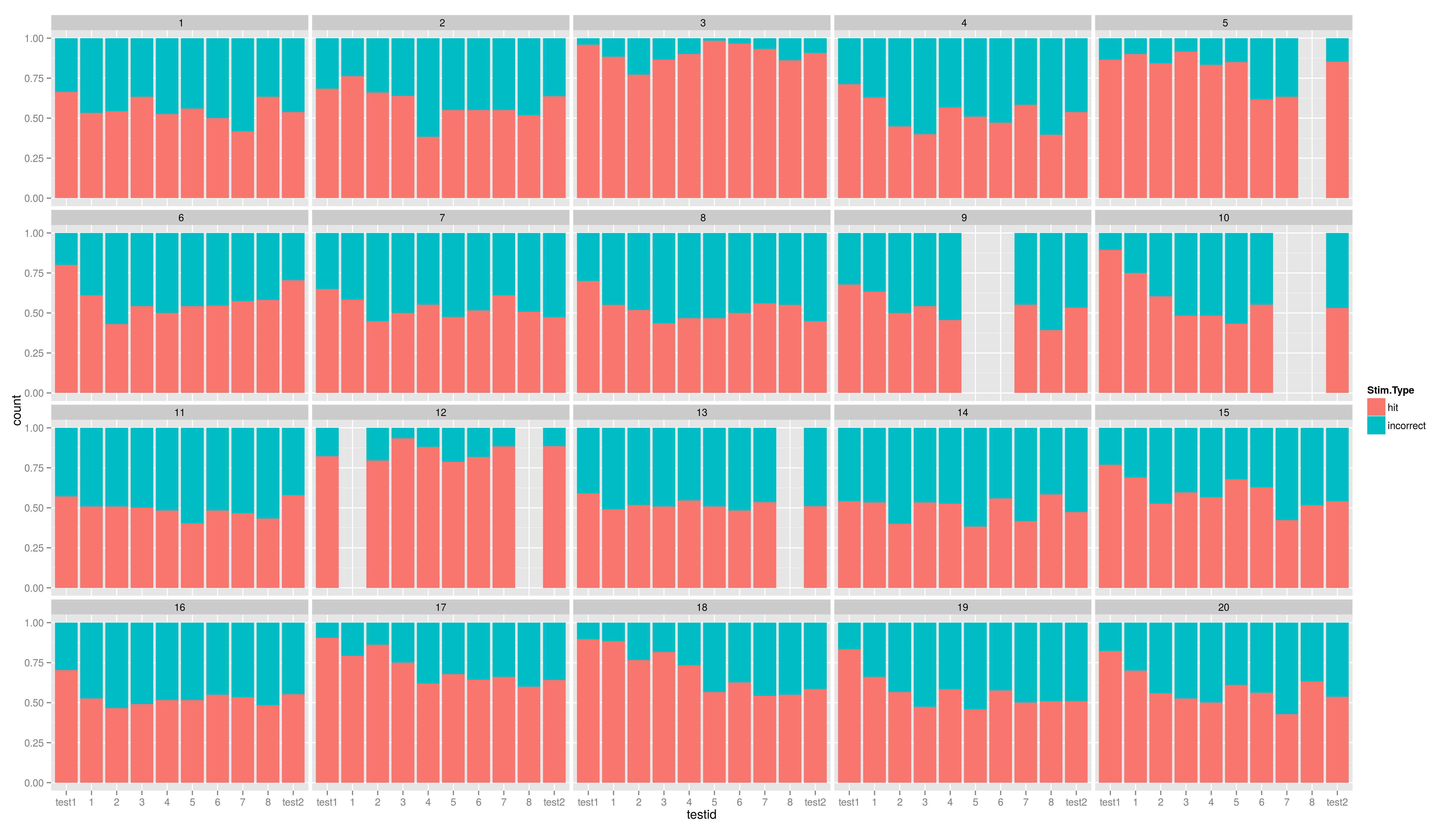
Summary Graphics

Just run the code and try to understand it. We will cover the ggplot graphics soon.

   1 > ggplot(data,aes(x=factor(Subject),fill=..count..)) +
   2 +     geom_bar() +
   3 +     facet_wrap(~testid)

so there are problems in coding of the test id
we remove the letters at the end using str_replace()

   1 > data$testid <- str_replace(data$testid,"[a-z]$","")
   2 > data$testid <- factor(data$testid,
   3 +                       levels=c("test1","1","2","3","4","5","6","7","8","test2"))
   4 > table(data$Subject,data$testid)
   5 test1  1  2  3  4  5  6  7  8 test2
   6 1     95 60 59 60 59 59 60 60 60    93
   7 2     95 59 59 58 60 60 60 60 60    91
   8 3     96 60 57 60 60 60 60 59 58    96
   9 4     94 54 58 60 60 55 53 60 58    93
  10 5     96 60 57 60 60 60 60 60  0    95
  11 6     95 59 58 59 58 59 55 54 55    95
  12 7     94 60 58 60 58 59 60 59 59    93
  13 8     90 60 54 55 60 60 60 59 60    96
  14 9     96 60 58 59 57  0  0 58 56    92

   1 > ggplot(data,aes(x=factor(Subject),fill=..count..)) +
   2 +     geom_bar() +
   3 +     facet_wrap(~testid)

And another one.

   1 > ggplot(data,aes(x=testid,fill=Stim.Type)) +
   2 +     geom_bar(position=position_fill()) +
   3 +     facet_wrap(~Subject)

RstatisTik/RstatisTikPortal/RcourSe/FinalFunction/CombMoreDataFrames (zuletzt geändert am 2015-05-01 13:08:47 durch mandy.vogel@googlemail.com)

-  ⇤ ← Revision 1 vom 2015-05-01 13:03:45 → 
  Größe: 15469
  Autor: mandy.vogel@googlemail.com
  Kommentar:
+   ← Revision 3 vom 2015-05-01 13:08:47 → ⇥
  Größe: 15175
  Autor: mandy.vogel@googlemail.com
  Kommentar:
-Gelöschter Text ist auf diese Art markiert.
+Hinzugefügter Text ist auf diese Art markiert.
 Zeile 175:
-== Reduce() Exercise ==
+=== solution ===
 Zeile 208:
-== Combine all data frames - exercise ==
+=== solution ===
 Zeile 250:
-== The Function no 2 ==
 Zeile 269:
-== The Subject column ==
 Zeile 280:
-== The Subject column ==
-Zeile 290:
+Zeile 289:
-== The Subject column ==
-Zeile 298:
+Zeile 296:
-== The Subject column ==
-Zeile 301:
+Zeile 298:
-== The Subject column ==
-Zeile 312:
+Zeile 308:
-== The Subject column Exercises ==
+=== solution ===
-Zeile 322:
+Zeile 318:
-== The Subject column Exercises ==
-Zeile 352:
+Zeile 348:
-[[attachment:graph1.png|{{attachment:graph1||width=800}}]]
== Summary Graphics ==
+[[attachment:graph1.png|{{attachment:graph1.png||width=800}}]]
-Zeile 372:
+Zeile 368:
-== Summary Graphics ==
-Zeile 381:
+Zeile 378:
-== Summary Graphics ==

Quick Links

Search Wiki

Page Tools

Introduction

Remember: Implicit Loops

Exercises

read one file

read several files

get files names

read in files

Result

Remember: Combining Data Frames

Reduce()

Example

Reduce() Exercise

solution

Combine all data frames

Combine all data frames - exercise

solution

The Function no 2

The Subject column

The Subject column Exercises

solution

Merging

Summary Graphics